Copula II — Definition
The word Copula derives from the Latin noun for a “link” or “tie” that connects two different things. When I talk about Copula in this post, actually I mean the Sklar’s Theorem.
Here is what the Sklar’s Theorem tells us: we always can find a Copula function \(C\) that every multivariate (a.k.a joint) cumulative distribution function(CDF) can be expressed by its marginal CDFs. In other words, we can use copula function to analyze the dependence between each random variable, and Sklar’s Theorem ensures such copula function exists.
Copula & Sklar’s Theorem
Definition: A \(\textbf{copula}\) is a function \(C: [0, 1]^n \rightarrow [0, 1]\) with the following properties:
For every \(u_1, u_2, \ldots, u_n \in [0, 1]\), \(C(1, 1, \ldots, u_i, \ldots, 1) = u_i\).
For every \(u_1, u_2, \ldots, u_n \in [0, 1]\), if any \(u_i = 0\), then \(C(u_1, u_2, \ldots, u_n) = 0\).
\(C\) is \(\textbf{n-increasing}\), meaning that for any \(a_1 \leq b_1, a_2 \leq b_2, \ldots, a_n \leq b_n\) in \([0, 1]\), the C-volume of the n-dimensional interval \([a_1, b_1] \times [a_2, b_2] \times \ldots \times [a_n, b_n]\) is nonnegative. That is, $$\begin{equation} \Delta C \geq 0, \end{equation}$$ where $\Delta C$ is the C-volume, a difference of values of $C$ that resembles a high-dimensional version of the finite difference.
Note: Given a copula $C: [0, 1]^n \rightarrow [0, 1]$, the $\Delta C$ for a box defined by the intervals $[a_1, b_1], [a_2, b_2], \ldots, [a_n, b_n]$ in $[0, 1]^n$ is calculated as follows: $$\begin{equation} \Delta C = \sum_{(i_1, i_2, \ldots, i_n) \in {0,1}^n} (-1)^{i_1 + i_2 + \cdots + i_n} C\left(b_1^{(i_1)}, b_2^{(i_2)}, \ldots, b_n^{(i_n)}\right), \end{equation}$$ where $b_j^{(i_j)} = a_j$ if $i_j = 0$ and $b_j^{(i_j)} = b_j$ if $i_j = 1$ for $1 \leq j \leq n$. This formula applies the inclusion-exclusion principle to calculate the volume under the copula over the specified box.
Consider a 2-dimensional copula $C: [0, 1]^2 \rightarrow [0, 1]$. To calculate the $\Delta C$ for a box in $[0, 1]^2$ defined by the intervals $[a_1, b_1]$ and $[a_2, b_2]$, we use the formula: \begin{equation} \Delta C = C(b_1, b_2) - C(a_1, b_2) - C(b_1, a_2) + C(a_1, a_2). \end{equation} This represents the inclusion-exclusion principle in 2 dimensions, ensuring that we correctly account for the volume under $C$ over the box by subtracting and adding the values of $C$ at the corners of the box.
In one word, we just want to make sure the volume inside the squre (\([0, 1] \times[0,1]\)) is positive. (Review the probability from joint CDF. For example, \(P(a_1<X<a_2, b_1<Y<b_2)\))
Sklar’s Theorem: For any joint distribution function \(H\) of random variables \(X_1, X_2, \ldots, X_n\) with marginal distribution functions \(F_1, F_2, \ldots, F_n\), there exists a copula \(C: [0, 1]^n \rightarrow [0, 1]\) such that for all \(x_1, x_2, \ldots, x_n\) in the extended real line (\(\overline{\mathbb{R}}\) or \(\mathbb{R} \cup \{-\infty,\infty\}\)), $$\begin{equation} H(x_1, x_2, \ldots, x_n) = C(F_1(x_1), F_2(x_2), \ldots, F_n(x_n)). \end{equation}$$ Furthermore, if the marginal distribution functions \(F_1, F_2, \ldots, F_n\) are continuous, then the copula \(C\) is unique. This means that the joint distribution \(H\) can be fully specified by its marginals and the copula \(C\).
Brief Proof: Currently, we only consider continuous case (CDF can be discontinuous, but that requires lots of math, and I don’t understand it 🙃. It I think is necessary, I may update in the future though I think continuous case is enough for most scenarios).
existence: Here, we use the definition of generalized inverse distribution function where
$$F^{-1}_X(y) = \inf\{x : F_X(x) \geq y\}, \quad 0 \leq y \leq 1.$$
By Probability Integral Transform, we know $U_i = F_i(X_i)$ is normally distributed on $[0,1]$ for $i = 1, 2,…,n$. We can easily construct copula function $C : [0, 1]^n \rightarrow [0, 1]$ s.t
$$C(u_1, u_2, …, u_n) = H(F^{-1}_1, F^{-1}_2,…, F^{-1}_n).$$
Here, $C(1,…,1,u_i,1,…,1) = u_i$ and $C(u_1,…,u_{i-1},0 ,u_{i+1},…,u_n) = 0$ are obvious because it just means marginal CDF or the probability of a single point, which is 0. Also, $C$ is $n$-increasing because we define it from CDFs, which is non-negative for sure.
uniqueness(skip): Simply because the continuous marginal CDF is one-to-one (bijective) function, so each copula has to follow same “mapping way” to connect marginal CDFs and joint CDF.
Type of Copulas
Theoretically, there are infinite types of Copula functions based on different distributions. I’ll introduce some common Copulas in bivariate distribution.
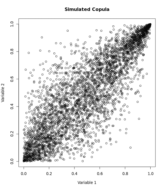
1, Gaussian Copula
- Symmetry: Gaussian copulas are symmetric, meaning they assign equal probability to joint tail events.
- No Tail Dependence: Gaussian copulas do not have tail dependence, implying that they underestimate the probability of extreme co-movements.
General Formula: $C(u,v;\theta) = \Phi_{\theta}(\Phi^{-1}(u), \Phi^{-1}(v))$
Conditional Copulas: $C_{2|1}^{-1}{ \alpha | u } = \Phi \left( \Phi^{-1}(\alpha) \sqrt{1-\theta^2} + \theta\Phi^{-1}(u) \right)$, $\theta \in [-1,1]$
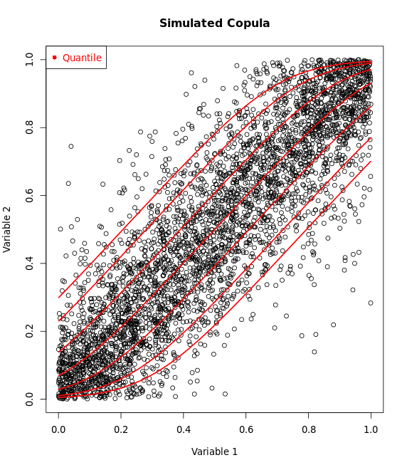
2, Gumbel Copula
- Asymmetry: The Gumbel copula is asymmetric, with more weight on the joint upper tails, capturing the events where both variables achieve high values together.
- Upper Tail Dependence: It exhibits upper tail dependence but not lower tail dependence.
General Formula: $C(u,v;\theta) = \exp\left( -\left[ (-\log u)^\theta + (-\log v)^\theta \right]^{1/\theta} \right)$
Conditional Copulas (Skip): Gumbel copula does not have an explicit expression. Instead, we may use numerical method to simulate.
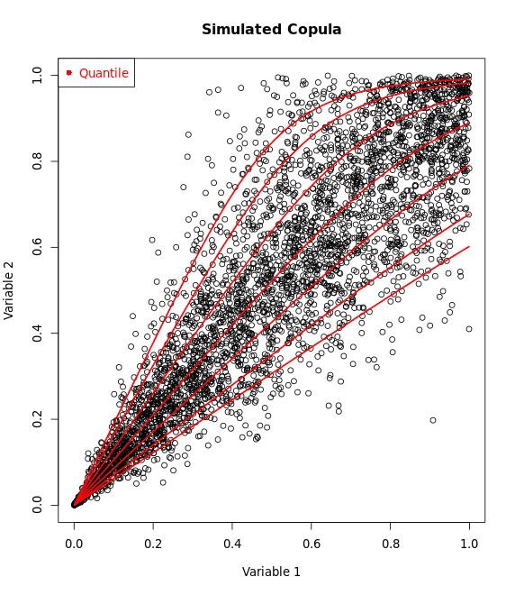
3, Clayton Copula
- Asymmetry: Clayton copulas are asymmetric, with more weight on the joint lower tails, indicating that they capture the events where both variables achieve low values together.
- Lower Tail Dependence: It exhibits strong lower tail dependence but no upper tail dependence.
General Formula: $C(u,v;\theta) = \left( u^{-\theta} + v^{-\theta} - 1 \right)^{-1/\theta}$
Conditional Copulas: $C_{2|1}^{-1}{ \alpha | u } = \left( \left(\alpha^{-\theta} - 1 \right) u^{-\theta} + 1 \right)^{-1/\theta}$, $1 \leq \theta < \infty$
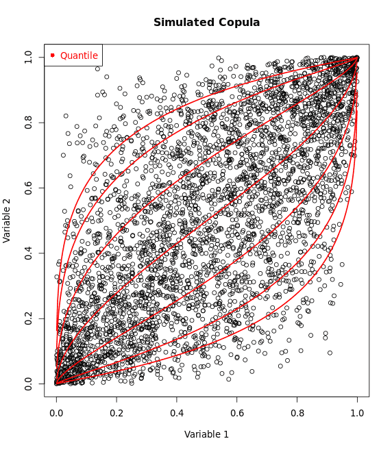
4, Frank Copula
- Symmetry: Frank copulas are symmetric, treating the dependence in the lower and upper tails equally.
- No Tail Dependence: Frank copulas do not exhibit tail dependence, similar to Gaussian copulas.
General Formula: $C(u,v;\theta) = -\frac{1}{\theta} \ln\left( 1 + \frac{(e^{-\theta u} - 1)(e^{-\theta v} - 1)}{e^{-\theta} - 1} \right)$
Conditional Copulas: $C_{2|1}^{-1}{ \alpha | u } = -\frac{1}{\theta} \ln \left( 1 - \frac{\alpha (1 - \exp(-\theta))}{\exp(-\theta u) + \alpha (1 - \exp(-\theta u))} \right)$, $\theta \in \mathbb{R} \backslash \{0\}$
Conclusion
Feel tedious, right? So, let’s just forget everything above, and just remember:
- “Copula(s)” refers a family of functions that help us understand how different things, like variables or data points, move together or relate to each other, despite having their own unique behaviors.
- Sklar’s Theorem ensures the existence and uniqueness of copulas for continuous marginal CDFs.
I also wanted to write some applications for Copulas, but I figured out that I’ve written too long for the boring mathematics stuff. Let’s finish this in the next post, and see you soon~